PLUMED Masterclass 21.4: Metadynamics

Origin

This masterclass was authored by Max Bonomi on March 1, 2021.

Aims

The aim of this Masterclass is to train users to perform and analyze a metadynamics simulation with PLUMED.

Objectives

Once this Masterclass is completed, users will be able to:

Write the PLUMED input file to perform metadynamics simulations.
Calculate the free energy as a function of the metadynamics collective variables.
Unbias metadynamics simulations.
Estimate the error in the reconstructed free energies using block analysis.
Assess the convergence of metadynamics simulations.
Recognize good from bad collective variables.

Overview of the theory

PLUMED can be used not only to analyze a pre-existing MD trajectory, but also to add forces on the CVs during a MD simulation, for example, in order to accelerate sampling. To this aim, we have implemented a variety of possible biases acting on CVs. The complete documentation for all the biasing methods available in PLUMED can be found at the page of the manual on biasing. In the following tutorial we will learn how to use PLUMED to perform and analyze a metadynamics simulation. Users are invited to familiarize with the theory behind this method by looking at one of the many reviews on this topic that are available. Some good places to look include:

Alessandrio Laio and Francesco Luigi Gervasio. Metadynamics: a method to simulate rare events and reconstruct the free energy in biophysics, chemistry and material science. Rep. Prog. Phys., 71:126601, 2008.
Alessandro Barducci, Massimiliano Bonomi, and Michele Parrinello. Metadynamics. Wiley Interdisciplinary Reviews: Computational Molecular Science, 1(5):826–843, 2011.
Ludovico Sutto, Simone Marsili, and Francesco Luigi Gervasio. New advances in metadynamics. Wiley Interdisciplinary Reviews: Computational Molecular Science, 2(5):771–779, 2012.
Giovanni Bussi, Davide Branduardi, and others. Free-energy calculations with metadynamics: Theory and practice. Rev. Comput. Chem, 28:1–49, 2015.

You can find a summary of the theory in this supplementary file..

Setting up the software

The users can refer to the procedures introduce in this masterclass and this masterclass to get instructions on how to install the required software. In this class, we will perform the simulations ourselves, so make sure that GROMACS code is properly installed.

Resources

The data needed to complete the exercises of this Masterclass can be found on GitHub. You can clone this repository locally on your machine using the following command:

git clone https://github.com/plumed/masterclass-21-4.git

This repositoy contains 3 folders:

data: GROMACS topology/PDB files for the two systems that we are going to simulate and python script for error analysis;
notebooks: Jupyter notebook to be used as template for the analysis of the PLUMED output;
slides: a brief presentation of the metadynamics theory.

To keep things clean, it is recommended to run each exercise in a separate sub-directory (i.e. Exercise-1, Exercise-2, …), which you can create inside the root directory masterclass-21-4. Students are invited to solve the exercises by themselves after completing the PLUMED input file templates provided below. In case of problems, students can rely on the solution notebook solution.ipynb provided in the GitHub repository.

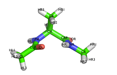
In many exercises, in the following tutorial we will play with a toy system, alanine dipeptide simulated in vacuo. An image of this molecule is shown below:

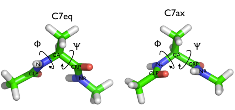
The molecule of the day: alanine dipeptide.

This rather simple molecule is useful to understand data analysis and free-energy methods. This system is a nice example because it presents two metastable states separated by a high free-energy barrier. It is conventional use to characterize the two states in terms of Ramachandran dihedral angles, which are denoted with $\phi$ (phi) and $\psi$ (psi) in the following figure:

Two metastable states of alanine dipeptide are characterized by their Ramachandran dihedral angles.

In the data/diala directory of the GitHub repository for this Masterclass, you will find two GROMACS .tpr files (topolA.tpr and topolB.tpr), which contain all the necessary information to perform a simulation starting from either one of the two metastable states of alanine dipeptide.

All the exercises have been tested with PLUMED version 2.7.0 and GROMACS 2019.6.

Exercises

Exercise 1: Familiarizing with alanine dipeptide

In this brief exercise, we will perform two 20 ns long standard MD simulations of alanine dipeptide starting from the two main metastable states of this system. To keep things clean, the users are invited to run these two simulations in two separate sub-folders. To run these simulations with GROMACS, please use the following commands:

# run this command in one directory
gmx mdrun -s topolA.tpr -nsteps 10000000
# and this in another one
gmx mdrun -s topolB.tpr -nsteps 10000000

After the simulations are completed, we can use PLUMED to monitor the behavior of the system. As you have learned in other masterclasses, PLUMED can compute and print collective variables (CVs) on a pre-calculated MD trajectory. Here, we will:

create a PLUMED input file with a text editor;
run the PLUMED driver utility;
visualize the output with the aid of a Jupyter notebook.

Let’s now prepare a PLUMED input file to calculate:

the value of the backbone dihedral $\phi$ ;
the value of the backbone dihedral $\psi$ .

by completing the template below (whenever you see an highlighted FILL string, this is a string that you must replace!):

Click on the labels of the actions for more information on what each action computes

# Activate MOLINFO functionalities
MOLINFOThis command is used to provide information on the molecules that are present in your system. More details STRUCTUREa file in pdb format containing a reference structure=__FILL__
# Compute the backbone dihedral angle phi, defined by atoms C-N-CA-C
# you should use MOLINFO shortcuts
The MOLINFO action with label  calculates somethingphi: TORSIONCalculate one or multiple torsional angles. More details ATOMSthe four atoms involved in the torsional angle=__FILL__
# Compute the backbone dihedral angle psi, defined by atoms N-CA-C-N
# here also you should to use MOLINFO shortcuts
The TORSION action with label phi calculates the following quantities: Quantity    Description  
phi.value the TORSION involving these atomspsi: TORSIONCalculate one or multiple torsional angles. More details ATOMSthe four atoms involved in the torsional angle=__FILL__
# Print the two collective variables on COLVAR file every step
The TORSION action with label psi calculates the following quantities: Quantity    Description  
psi.value the TORSION involving these atomsPRINTPrint quantities to a file. More details ARGthe labels of the values that you would like to print to the file=__FILL__ FILEthe name of the file on which to output these quantities=COLVAR STRIDE the frequency with which the quantities of interest should be output=__FILL__

# Activate MOLINFO functionalities
MOLINFOThis command is used to provide information on the molecules that are present in your system. More details STRUCTUREa file in pdb format containing a reference structure=../data/diala/dialaA.pdb 
# Compute the backbone dihedral angle phi, defined by atoms C-N-CA-C
# you should use MOLINFO shortcuts
The MOLINFO action with label  calculates somethingphi: TORSIONCalculate one or multiple torsional angles. More details ATOMSthe four atoms involved in the torsional angle=@phi-2the four atoms that are required to calculate the phi dihedral for residue 2. Click here for more information. 
# Compute the backbone dihedral angle psi, defined by atoms N-CA-C-N
# here also you should to use MOLINFO shortcuts
The TORSION action with label phi calculates the following quantities: Quantity    Description  
phi.value the TORSION involving these atomspsi: TORSIONCalculate one or multiple torsional angles. More details ATOMSthe four atoms involved in the torsional angle=@psi-2the four atoms that are required to calculate the psi dihedral for residue 2. Click here for more information. 
# Print the two collective variables on COLVAR file every step
The TORSION action with label psi calculates the following quantities: Quantity    Description  
psi.value the TORSION involving these atomsPRINTPrint quantities to a file. More details ARGthe labels of the values that you would like to print to the file=phi,psi FILEthe name of the file on which to output these quantities=COLVAR STRIDE the frequency with which the quantities of interest should be output=1

Once your plumed.dat file is complete, you can run the PLUMED driver on the two MD trajectories as follows:

plumed driver --plumed plumed.dat --mf_xtc traj_comp.xtc

The two COLVAR files can be analyzed using the Jupyter notebook plumed-pandas.ipynb provided in the folder notebooks. This notebook allows you to import a COLVAR file produced by PLUMED and to generate the desired figures using the matplotlib library. The users are invited to:

inspect the dynamics of the two backbone dihedrals in the two separate simulations;
calculate the fluctuations (standard deviation) of the two CVs in the different basins visited.

Are both simulations long enough to visit all the relevant conformations or instead they remain trapped in different regions of the $\phi$ / $\psi$ space?

Exercise 2: My first metadynamics simulation

In this exercise we will setup and perform a well-tempered metadynamics run using the backbone dihedral $\phi$ as collective variable. During the calculation, we will also monitor the behavior of the other backbone dihedral $\psi$ . Here you can find a sample plumed.dat file that you can use as a template.

Click on the labels of the actions for more information on what each action computes

# Activate MOLINFO functionalities
MOLINFOThis command is used to provide information on the molecules that are present in your system. More details STRUCTUREa file in pdb format containing a reference structure=__FILL__
# Compute the backbone dihedral angle phi, defined by atoms C-N-CA-C
# you should use MOLINFO shortcuts 
The MOLINFO action with label  calculates somethingphi: TORSIONCalculate one or multiple torsional angles. More details ATOMSthe four atoms involved in the torsional angle=__FILL__
# Compute the backbone dihedral angle psi, defined by atoms N-CA-C-N
# here also you should to use MOLINFO shortcuts 
The TORSION action with label phi calculates the following quantities: Quantity    Description  
phi.value the TORSION involving these atomspsi: TORSIONCalculate one or multiple torsional angles. More details ATOMSthe four atoms involved in the torsional angle=__FILL__
# Activate well-tempered metadynamics in phi
The TORSION action with label psi calculates the following quantities: Quantity    Description  
psi.value the TORSION involving these atomsmetad: METADUsed to performed metadynamics on one or more collective variables. More details ARGthe labels of the scalars on which the bias will act=__FILL__ ...
# Deposit a Gaussian every 500 time steps, with initial height 
# equal to 1.2 kJ/mol and bias factor equal to 8
  PACEthe frequency for hill addition=500 HEIGHTthe heights of the Gaussian hills=1.2 BIASFACTORuse well tempered metadynamics and use this bias factor=8
# Gaussian width (sigma) should be chosen based on the CV fluctuations in unbiased run
# try 1/2 or 1/3 of the estimated fluctuations
  SIGMAthe widths of the Gaussian hills=__FILL__
# Gaussians will be written to file and also stored on grid
  FILE a file in which the list of added hills is stored=HILLS GRID_MINthe lower bounds for the grid=-pi GRID_MAXthe upper bounds for the grid=pi
...
# Print both collective variables on COLVAR file every 10 steps
The METAD action with label metad calculates the following quantities: Quantity    Description  
metad.bias the instantaneous value of the bias potentialPRINTPrint quantities to a file. More details ARGthe labels of the values that you would like to print to the file=__FILL__ FILEthe name of the file on which to output these quantities=COLVAR STRIDE the frequency with which the quantities of interest should be output=__FILL__

# Activate MOLINFO functionalities
MOLINFOThis command is used to provide information on the molecules that are present in your system. More details STRUCTUREa file in pdb format containing a reference structure=../data/diala/dialaA.pdb
# Compute the backbone dihedral angle phi, defined by atoms C-N-CA-C
# you should use MOLINFO shortcuts
The MOLINFO action with label  calculates somethingphi: TORSIONCalculate one or multiple torsional angles. More details ATOMSthe four atoms involved in the torsional angle=@phi-2the four atoms that are required to calculate the phi dihedral for residue 2. Click here for more information. 
# Compute the backbone dihedral angle psi, defined by atoms N-CA-C-N
# here also you should to use MOLINFO shortcuts
The TORSION action with label phi calculates the following quantities: Quantity    Description  
phi.value the TORSION involving these atomspsi: TORSIONCalculate one or multiple torsional angles. More details ATOMSthe four atoms involved in the torsional angle=@psi-2the four atoms that are required to calculate the psi dihedral for residue 2. Click here for more information. 
# Activate well-tempered metadynamics in phi
The TORSION action with label psi calculates the following quantities: Quantity    Description  
psi.value the TORSION involving these atomsmetad: METADUsed to performed metadynamics on one or more collective variables. More details ARGthe labels of the scalars on which the bias will act=phi ...
# Deposit a Gaussian every 500 time steps, with initial height
# equal to 1.2 kJ/mol and bias factor equal to 8
  PACEthe frequency for hill addition=500 HEIGHTthe heights of the Gaussian hills=1.2 BIASFACTORuse well tempered metadynamics and use this bias factor=8
# Gaussian width (sigma) should be chosen based on the CV fluctuations in unbiased run
# try 1/2 or 1/3 of the estimated fluctuations
  SIGMAthe widths of the Gaussian hills=0.3
# Gaussians will be written to file and also stored on grid
  FILE a file in which the list of added hills is stored=HILLS GRID_MINthe lower bounds for the grid=-pi GRID_MAXthe upper bounds for the grid=pi
...
# Print both collective variables on COLVAR file every 10 steps
The METAD action with label metad calculates the following quantities: Quantity    Description  
metad.bias the instantaneous value of the bias potentialPRINTPrint quantities to a file. More details ARGthe labels of the values that you would like to print to the file=phi,psi FILEthe name of the file on which to output these quantities=COLVAR STRIDE the frequency with which the quantities of interest should be output=10

Once your plumed.dat file is complete, you can run a 20 ns long metadynamics simulations starting from either of the two provided conformations, for example topolA.tpr. All you need to do is execute the following command:

gmx mdrun -s topolA.tpr -nsteps 10000000 -plumed plumed.dat

During the metadynamics simulation, PLUMED will create two files, named COLVAR and HILLS. The COLVAR file contains all the information specified by the PRINT command, in this case the value of the backbone dihedrals $\phi$ and $\psi$ every 10 steps of simulation. The HILLS file contains a list of the Gaussian kernels deposited along the simulation.

Let’s visualize the time series of the two collective variables. Take your time to inspect the behavior of the two CVs. What are the main differences with respect to the trajectories you produced from the first exercise?

At this point, we can estimate the free energy as a function of the metadynamics CV directly from the metadynamics bias potential. In order to do so, the utility sum_hills can be used to sum the Gaussian kernels deposited during the simulation and stored in the HILLS file. To calculate the free energy as a function of $\phi$ , it is sufficient to use the following command:

plumed sum_hills --hills HILLS

The command above generates a file called fes.dat in which the free-energy surface as function of $\phi$ is calculated on a regular grid. One can modify the default name for the free-energy file, as well as the boundaries and bin size of the grid, by using the following sum_hills options:

--outfile - specify the outputfile for sumhills
--min - the lower bounds for the grid
--max - the upper bounds for the grid
--bin - the number of bins for the grid
--spacing - grid spacing, alternative to the number of bins

To give a preliminary assessment of the convergence of a metadynamics simulation, one can calculate the estimate of the free energy as a function of simulation time. At convergence, the reconstructed profiles should be similar. The sum_hills option --stride should be used to give an estimate of the free energy every N Gaussian kernels deposited, and the option --mintozero can be used to align the profiles by setting the global minimum to zero. If we use the following command:

plumed sum_hills --hills HILLS --stride 200 --mintozero

one free energy is calculated every 200 Gaussian kernels deposited, and the global minimum is set to zero in all profiles. Now, you can visualize the free-energy estimate as a function of simulation time and assess how it changed during the course of the simulation. In the last part of this 20 ns long metadynamics simulation, the free-energy estimate should not change significantly.

Looking at the time-evolution of the entire free-energy profile might not be straightforward. Therefore, what we usually do is focusing on a few metastable states, or local free-energy minima, and calculating their estimated free-energy difference as a function of time. In case of alanine dipeptide, this is rather easy since there are only two major states in the free-energy profile as a function of the CV $\phi$ .

The users should now:

calculate from the estimate of the free energy $F(\phi)$ at a given simulation time, the difference in free energy between the two basins. In order to do this, you should define a reasonable interval around the two local free-energy minima and recall that the probability of this state is the integral of the probability $P(\phi)= exp(-F(\phi)/k_BT)$ in the chosen interval;
plot the estimated free-energy difference as a function of simulation time.

These two observations:

the system is diffusing rapidly in the entire CV space
the estimated free energy does not significantly change as a function of time

are two indications that the simulation might have converged.

IMPORTANT: The two conditions listed above are necessary, but not sufficient to declare convergence. We will learn below how to perform a quantitative analysis of the convergence of a metadynamics simulation.

Exercise 3: Reweighting (unbiasing) a metadynamics simulation

In the previous exercise we biased $\phi$ and computed the free energy as a function of the same variable directly from the metadynamics bias potential using the sum_hills utility. However, in many cases you might decide which variable should be analyzed after having performed a metadynamics simulation. For example, you might want to calculate the free energy as a function of CVs other than those biased during the metadynamics simulation, such as the dihedral $\psi$ . At variance with standard MD simulations, you cannot simply calculate histograms of other variables directly from your metadynamics trajectory, because the presence of the metadynamics bias potential has altered the statistical weight of each frame. To remove the effect of this bias and thus be able to calculate properties of the system in the unbiased ensemble, you must reweight (unbias) your simulation.

There are multiple ways to calculate the correct statistical weight of each frame in your metadynamics trajectory and thus to reweight your simulation. For example:

weights can be calculated by considering the time-dependence of the metadynamics bias potential as discussed in this paper.
weights can be calculated using the metadynamics bias potential obtained at the end of the simulation and assuming a constant bias during the entire course of the simulation as discussed in this paper.

In this exercise we will use the second method, which is identical to the umbrella-sampling reweighting approach that you may have come across in other masterclasses. In order to compute the weights we will use the driver tool.

First of all, you need to prepare a plumed_reweight.dat file that is identical to the one you used for running your metadynamics simulation except for a few modifications:

you need to add the keyword RESTART=YES to the METAD command. This will make this action behave as if PLUMED was restarting, i.e. PLUMED will read from the HILLS file the Gaussians that have previously been accumulated;
you need to set the Gaussian HEIGHT to zero and the PACE to a large number. This will actually avoid adding new Gaussians (and even if they are added they will have zero height);
you need to modify the PRINT statement so that you write every frame and that, in addition to phi and psi, you also write metad.bias;
you might also want to change the name of the output file to COLVAR_REWEIGHT.

Here how the plumed_reweight.dat should look like:

Click on the labels of the actions for more information on what each action computes

# Activate MOLINFO functionalities
MOLINFOThis command is used to provide information on the molecules that are present in your system. More details STRUCTUREa file in pdb format containing a reference structure=__FILL__

__FILL__ # here goes the definitions of the phi and psi CVs

# Activate well-tempered metadynamics in phi
The MOLINFO action with label  calculates somethingmetad: METADUsed to performed metadynamics on one or more collective variables. More details ARGthe labels of the scalars on which the bias will act=__FILL__ ...
# Deposit a Gaussian every 10000000 time steps (never!), with initial height equal to 0.0 kJ/mol
  PACEthe frequency for hill addition=10000000 HEIGHTthe heights of the Gaussian hills=0.0 # <- this is the new stuff!
# The bias factor and Gaussian width are the same as before
  BIASFACTORuse well tempered metadynamics and use this bias factor=__FILL__ SIGMAthe widths of the Gaussian hills=__FILL__
# Gaussians will be read from file and stored on grid
# Make sure you specify the path the HILLS file produced in Exercise 2!
  FILE a file in which the list of added hills is stored=HILLS GRID_MINthe lower bounds for the grid=-pi GRID_MAXthe upper bounds for the grid=pi
# Say that METAD should be restarting (= reading an existing HILLS file)
  RESTARTallows per-action setting of restart (YES/NO/AUTO)=YES # <- this is the new stuff!
...

# Print out the values of phi, psi and the metadynamics bias potential
# Make sure you print out the 3 variables in the specified order at every step
The METAD action with label metad calculates the following quantities: Quantity    Description  
metad.bias the instantaneous value of the bias potentialPRINTPrint quantities to a file. More details ARGthe labels of the values that you would like to print to the file=__FILL__ FILEthe name of the file on which to output these quantities=COLVAR_REWEIGHT STRIDE the frequency with which the quantities of interest should be output=__FILL__  # <- also change this one!

# Activate MOLINFO functionalities
MOLINFOThis command is used to provide information on the molecules that are present in your system. More details STRUCTUREa file in pdb format containing a reference structure=../data/diala/dialaA.pdb

# here goes the definitions of the phi and psi CVs
The MOLINFO action with label  calculates somethingphi: TORSIONCalculate one or multiple torsional angles. More details ATOMSthe four atoms involved in the torsional angle=@phi-2the four atoms that are required to calculate the phi dihedral for residue 2. Click here for more information. 
The TORSION action with label phi calculates the following quantities: Quantity    Description  
phi.value the TORSION involving these atomspsi: TORSIONCalculate one or multiple torsional angles. More details ATOMSthe four atoms involved in the torsional angle=@psi-2the four atoms that are required to calculate the psi dihedral for residue 2. Click here for more information. 

# Activate well-tempered metadynamics in phi
The TORSION action with label psi calculates the following quantities: Quantity    Description  
psi.value the TORSION involving these atomsmetad: METADUsed to performed metadynamics on one or more collective variables. More details ARGthe labels of the scalars on which the bias will act=phi ...
# Deposit a Gaussian every 10000000 time steps (never!), with initial height equal to 0.0 kJ/mol
  PACEthe frequency for hill addition=10000000 HEIGHTthe heights of the Gaussian hills=0.0 # <- this is the new stuff!
# The bias factor and Gaussian width are the same as before
  BIASFACTORuse well tempered metadynamics and use this bias factor=8 SIGMAthe widths of the Gaussian hills=0.3
# Gaussians will be read from file and stored on grid
# Make sure you specify the path the HILLS file produced in Exercise 2!
  FILE a file in which the list of added hills is stored=../work/FAKE_HILLS GRID_MINthe lower bounds for the grid=-pi GRID_MAXthe upper bounds for the grid=pi
# Say that METAD should be restarting (= reading an existing HILLS file)
  RESTARTallows per-action setting of restart (YES/NO/AUTO)=YES # <- this is the new stuff!
...

# Print out the values of phi, psi and the metadynamics bias potential
# Make sure you print out the 3 variables in the specified order at every step
The METAD action with label metad calculates the following quantities: Quantity    Description  
metad.bias the instantaneous value of the bias potentialPRINTPrint quantities to a file. More details ARGthe labels of the values that you would like to print to the file=phi,psi FILEthe name of the file on which to output these quantities=COLVAR_REWEIGHT STRIDE the frequency with which the quantities of interest should be output=10  # <- also change this one!

Now you can run the driver tool using this command:

plumed driver --mf_xtc traj_comp.xtc --plumed plumed_reweight.dat --kt 2.494339

where traj_comp.xtc is the metadynamics trajectory produced in exercise 2. Notice that you have to specify the value of $k_BT$ in energy units. While running your simulation this information was communicated by the MD code.

As a result, PLUMED will produce a new COLVAR_REWEIGHT file with one additional column containing the metadynamics bias potential $V(s)$ calculated using all the Gaussians deposited along the entire trajectory. You can easily obtain the weight $w$ of each frame using the expression $w\propto\exp\left(\frac{V(s)}{k_BT}\right)$ (umbrella-sampling-like reweighting). At this point, you can read the COLVAR_REWEIGHT file using a python notebook and compute a weighted histogram or, alternatively, if you want PLUMED to do the weighted histograms for you, you can add the following lines at the end of the plumed_reweight.dat file and re-run PLUMED driver:

Click on the labels of the actions for more information on what each action computes

# Use the metadynamics bias as argument
as: REWEIGHT_BIASCalculate weights for ensemble averages that negate the effect the bias has on the region of phase space explored More details ARG the biases that must be taken into account when reweighting=__FILL__

# Calculate histograms of phi and psi dihedrals every 50 steps
# using the weights obtained from the metadynamics bias potentials (umbrella-sampling-like reweighting)
# Look at the manual to understand the parameters of the HISTOGRAM action!
The REWEIGHT_BIAS action with label as calculates the following quantities: Quantity    Description  
as.value the weight to use for this frame to negate the effect the biashhphi: HISTOGRAMAccumulate the average probability density along a few CVs from a trajectory. More details ARGthe quantities that are being used to construct the histogram=phi STRIDE the frequency with which to store data for averaging=50 GRID_MIN the lower bounds for the grid=-pi GRID_MAX the upper bounds for the grid=pi GRID_BINthe number of bins for the grid=50 BANDWIDTHthe bandwidths for kernel density esimtation=0.05 LOGWEIGHTSthe logarithm of the quantity to use as the weights when calculating averages=as
The HISTOGRAM action with label hhphi calculates the following quantities: Quantity    Description  
hhphi.value the estimate of the histogram as a function of the argument that was obtainedhhpsi: HISTOGRAMAccumulate the average probability density along a few CVs from a trajectory. More details ARGthe quantities that are being used to construct the histogram=psi STRIDE the frequency with which to store data for averaging=50 GRID_MIN the lower bounds for the grid=-pi GRID_MAX the upper bounds for the grid=pi GRID_BINthe number of bins for the grid=50 BANDWIDTHthe bandwidths for kernel density esimtation=0.05 LOGWEIGHTSthe logarithm of the quantity to use as the weights when calculating averages=as

# Convert histograms h(s) to free energies F(s) = -kBT * log(h(s))
The HISTOGRAM action with label hhpsi calculates the following quantities: Quantity    Description  
hhpsi.value the estimate of the histogram as a function of the argument that was obtainedffphi: CONVERT_TO_FESConvert a histogram to a free energy surface. More details GRIDthe histogram that you would like to convert into a free energy surface (old syntax)=hhphi
The CONVERT_TO_FES action with label ffphi calculates the following quantities: Quantity    Description  
ffphi.value the free energy surfaceffpsi: CONVERT_TO_FESConvert a histogram to a free energy surface. More details GRIDthe histogram that you would like to convert into a free energy surface (old syntax)=hhpsi

# Print out the free energies F(s) to file once the entire trajectory is processed 
The CONVERT_TO_FES action with label ffpsi calculates the following quantities: Quantity    Description  
ffpsi.value the free energy surfaceDUMPGRIDOutput the function on the grid to a file with the PLUMED grid format. More details GRIDthe grid you would like to print (can also use ARG for specifying what is being printed)=ffphi FILE the file on which to write the grid=ffphi.dat
The DUMPGRID action with label  calculates somethingDUMPGRIDOutput the function on the grid to a file with the PLUMED grid format. More details GRIDthe grid you would like to print (can also use ARG for specifying what is being printed)=ffpsi FILE the file on which to write the grid=ffpsi.dat

# Activate MOLINFO functionalities
MOLINFOThis command is used to provide information on the molecules that are present in your system. More details STRUCTUREa file in pdb format containing a reference structure=../data/diala/dialaA.pdb 
# Compute the backbone dihedral angle phi, defined by atoms C-N-CA-C
# you should use MOLINFO shortcuts
The MOLINFO action with label  calculates somethingphi: TORSIONCalculate one or multiple torsional angles. More details ATOMSthe four atoms involved in the torsional angle=@phi-2the four atoms that are required to calculate the phi dihedral for residue 2. Click here for more information.  
# Compute the backbone dihedral angle psi, defined by atoms N-CA-C-N
# here also you should to use MOLINFO shortcuts
The TORSION action with label phi calculates the following quantities: Quantity    Description  
phi.value the TORSION involving these atomspsi: TORSIONCalculate one or multiple torsional angles. More details ATOMSthe four atoms involved in the torsional angle=@psi-2the four atoms that are required to calculate the psi dihedral for residue 2. Click here for more information.  
# Activate well-tempered metadynamics in phi
The TORSION action with label psi calculates the following quantities: Quantity    Description  
psi.value the TORSION involving these atomsmetad: METADUsed to performed metadynamics on one or more collective variables. More details ARGthe labels of the scalars on which the bias will act=phi ...
   # Deposit a Gaussian every 10000000 time steps (never!), with initial height equal to 0.0 kJ/mol 
   PACEthe frequency for hill addition=10000000 HEIGHTthe heights of the Gaussian hills=0.0 BIASFACTORuse well tempered metadynamics and use this bias factor=8# <- this is the new stuff! 
   # Gaussian width (sigma) should be chosen based on the CV fluctuations in unbiased run 
   SIGMAthe widths of the Gaussian hills=0.3 
   # Gaussians will be written to file and also stored on grid 
   FILE a file in which the list of added hills is stored=../work/FAKE_HILLS GRID_MINthe lower bounds for the grid=-pi GRID_MAXthe upper bounds for the grid=pi
   # Say that METAD should be restarting (= reading an existing HILLS file) 
   RESTARTallows per-action setting of restart (YES/NO/AUTO)=YES # <- this is the new stuff! 
...

# Use the metadynamics bias as argument
The METAD action with label metad calculates the following quantities: Quantity    Description  
metad.bias the instantaneous value of the bias potentialas: REWEIGHT_BIASCalculate weights for ensemble averages that negate the effect the bias has on the region of phase space explored More details ARG the biases that must be taken into account when reweighting=metad.bias

# Calculate histograms of phi and psi dihedrals every 50 steps
# using the weights obtained from the metadynamics bias potentials (umbrella-sampling-like reweighting)
# Look at the manual to understand the parameters of the HISTOGRAM action!
The REWEIGHT_BIAS action with label as calculates the following quantities: Quantity    Description  
as.value the weight to use for this frame to negate the effect the biashhphi: HISTOGRAMAccumulate the average probability density along a few CVs from a trajectory. More details ARGthe quantities that are being used to construct the histogram=phi STRIDE the frequency with which to store data for averaging=50 GRID_MIN the lower bounds for the grid=-pi GRID_MAX the upper bounds for the grid=pi GRID_BINthe number of bins for the grid=50 BANDWIDTHthe bandwidths for kernel density esimtation=0.05 LOGWEIGHTSthe logarithm of the quantity to use as the weights when calculating averages=as
The HISTOGRAM action with label hhphi calculates the following quantities: Quantity    Description  
hhphi.value the estimate of the histogram as a function of the argument that was obtainedhhpsi: HISTOGRAMAccumulate the average probability density along a few CVs from a trajectory. More details ARGthe quantities that are being used to construct the histogram=psi STRIDE the frequency with which to store data for averaging=50 GRID_MIN the lower bounds for the grid=-pi GRID_MAX the upper bounds for the grid=pi GRID_BINthe number of bins for the grid=50 BANDWIDTHthe bandwidths for kernel density esimtation=0.05 LOGWEIGHTSthe logarithm of the quantity to use as the weights when calculating averages=as

# Convert histograms h(s) to free energies F(s) = -kBT * log(h(s))
The HISTOGRAM action with label hhpsi calculates the following quantities: Quantity    Description  
hhpsi.value the estimate of the histogram as a function of the argument that was obtainedffphi: CONVERT_TO_FESConvert a histogram to a free energy surface. More details GRIDthe histogram that you would like to convert into a free energy surface (old syntax)=hhphi
The CONVERT_TO_FES action with label ffphi calculates the following quantities: Quantity    Description  
ffphi.value the free energy surfaceffpsi: CONVERT_TO_FESConvert a histogram to a free energy surface. More details GRIDthe histogram that you would like to convert into a free energy surface (old syntax)=hhpsi

# Print out the free energies F(s) to file once the entire trajectory is processed
The CONVERT_TO_FES action with label ffpsi calculates the following quantities: Quantity    Description  
ffpsi.value the free energy surfaceDUMPGRIDOutput the function on the grid to a file with the PLUMED grid format. More details GRIDthe grid you would like to print (can also use ARG for specifying what is being printed)=ffphi FILE the file on which to write the grid=ffphi.dat
DUMPGRIDOutput the function on the grid to a file with the PLUMED grid format. More details GRIDthe grid you would like to print (can also use ARG for specifying what is being printed)=ffpsi FILE the file on which to write the grid=ffpsi.dat

You can now compare the free energies as a function of $\phi$ calculated:

directly from the metadynamics bias potential using sum_hills as done in exercise 2;
using the reweighting procedure introduced in this exercise.

Are the two free energies identical?

Exercise 4: Estimating the error in free energies using block-analysis

In the previous exercise, we calculated the final bias $V(s)$ on the entire metadynamics trajectory and we used this quantity to calculate the correct statistical weight of each frame, which is needed to reweight the biased simulation. In this exercise, the user will learn how this information can be used to calculate the error in the reconstructed free energies and assess whether the simulation is converged or not.

Let’s first:

calculate the un-biasing weights $w\propto\exp\left(\frac{V(s)}{k_BT}\right)$ from the COLVAR_REWEIGHT file obtained at the end of exercise 3;
print them in a file (called for example phi.weight) containing the value of the dihedral $\phi$ and the corresponding (un-normalized) weight $w$ for each frame of the metadynamics trajectory.

At this point we can apply the block-analysis technique (for more info about the theory, have a look at other masterclasses) to calculate the average free energy across the blocks and the error as a function of block size. For your convenience, the do_block_fes.py python script provided in the data directory of the GitHub repository of this Masterclass can be used to read the phi.weight file and produce the desired output. The users should properly choose the following input parameters:

# Arguments of do_block_fes.py
# - FILE: input file with 2 colums containing the CV value and weight for each frame of the trajectory
# - NCV: number of CVs
# - MIN/MAX: CV range
# - NBIN: # points in output free energy
# - KBT: temperature in energy units (kJoule/mol)
# - N: Block size
# 
python3 do_block_fes.py FILE NCV MIN MAX NBIN KBT N

and run the above script for different block sizes ranging from 1 to 1000. For each choice of block size, the script will produce an output file, which contains 3 colums:

the value of the $\phi$ variable on a grid;
the free energy averaged across the blocks for each point of the grid;
the associated error for each point of the grid.

At this point, the users should:

calculate the average error across the free-energy profile, i.e. the grid points, for each block size chosen;
visualize this average error as a function of the block size.

The users should verify that the error increases with the block size (why?) until it reaches a plateau when the dimension of the block exceeds the correlation time between data points. If a plateau is not observed, then the simulation is not converged yet and should be run a bit longer.

From this analysis, what can we say about the convergence of the metadynamics simulation performed in exercise 2?

Exercise 5: Recognizing good from bad CVs

In the previous exercises, we have performed a metadynamics simulation on alanine dipeptide using the backbone dihedral $\phi$ as CV. We have analyzed the simulation and noticed that:

under the effect of the bias potential, the system rapidly diffuses in the entire CV space;
the error in the reconstructed free energy calculated with block analysis rapidly reaches a plateau.

These two observations indicate that our simulation is converged and that the dihedral $\phi$ can be considered a good CV. A good set of CVs for metadynamics should:

discriminate between the relevant metastable states of the system;
include all the slow modes that characterize transitions between such states;
be as small as possible.

Identifying a priori a good set of CVs to describe a specific problem is far from trivial. In this exercise, the users will learn how to detect potential problems in their choice of CV(s). Let’s first perform additional 1D metadynamics simulations using one of the following CVs:

the dihedral $\psi$ ;
the radius of gyration, defined on all the heavy atoms of the system;
the distance between Oxigen atom 6 and Hydrogen atom 8.

The users are invited to prepare, for each of the CV listed above, a PLUMED input file to perform a 1D well-tempered metadynamics simulation, execute the simulation, and analyse the results in terms of:

diffusion of the system in the space of the dihedral $\phi$
error analysis in the free energy as a function of $\phi$

and compare the results with the previous simulation in which $\phi$ was used as the metadynamics CV. Based on this analysis, can you discriminate between good from bad CVs?

To complete this exercise, the users should define and test a new CV that is either:

as good as the dihedral $\phi$ ;
the worst possible CV to accelerate sampling and describe the two main conformational states of alanine dipeptide.

Please post the results of your simulations on Slack!

Exercise 6: A ‘real-life’ application

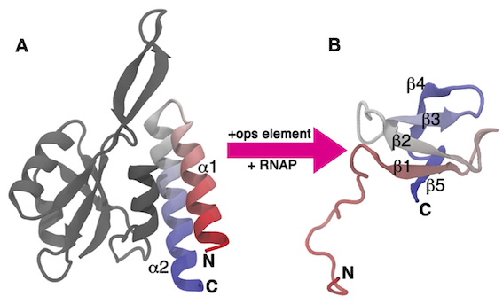
In this last exercise, we will tackle a real-life biological problem: studying the conformational transition of a complex biological system. The system that we are going to study is the C-terminal domain (CTD) of the RfaH virulence factor from Escherichia coli. As shown in the figure below, this part of the system, which we refer to as RfaH-CTD, undergoes a dramatic conformational transformation from β-barrel to α-helical, which is stabilized by the N-terminal domain of the RfaH virulence factor.

In the data/RfaH-CTD folder of the GitHub repository of this Masterclass, you will find:

two PDB files of RfaH-CTD in the α-helical and β-barrel states;
a topol.tpr file, which is needed to perform a MD simulation of this sytem with GROMACS.

The objective of this exercises are to:

compute the free-energy difference between the α-helical and β-barrel states of RfaH-CTD (with error estimate);
(optional) determine the structure and population of other metastable states, if present.

In order to complete the exercise, the students should:

choose their own CVs (maximum 3) and perform a well-tempered metadynamics simulation. Any CV natively implemented in PLUMED (see here) or defined by the users directly in the input file (see CUSTOM) can be used;
monitor the RMSD of the system from the two reference conformations during the course of the simulation;
analyze the results as done in the previous exercises (assessment of convergence and error analysis);
report the free energies (with error bar) as a function of the two RMSD CVs calculated with respect to the reference PDBs;
(optional) report structure and population of the most signicant, i.e. populated, states.

Please keep in mind that:

we are simulating the system using a simplified, structure-based potential, called SMOG. SMOG is significantly less computational demanding than all-atoms, explicit solvent force fields. However, the simulation of this system might take a few hours, so allocate enough time to complete this exercise;
some of the CVs or PLUMED functionalities might not work as hydrogen atoms are not present in the system. However, there is always a way around this, so be creative;
due to the nature of the force field, we are simulating at an unphysical temperature of 60K. Be ready to test large values of the BIASFACTOR.

Finally, due to the special nature of the force field, please execute GROMACS using the following command:

gmx mdrun -plumed plumed.dat -ntomp 4 -noddcheck

You can adjust the number of CPU cores you want to use (here 4, OpenMP parallelization), based on the available resources. The system is not particularly big, therefore using a large number of cores might be inefficient.

Please post the results of your simulations on Slack!

PLUMED-TUTORIALS

A collaborative, community-driven learning ecosystem

PLUMED Masterclass 21.4: Metadynamics

Origin

Aims

Objectives

Overview of the theory

Setting up the software

Resources

Exercises

Exercise 1: Familiarizing with alanine dipeptide

Exercise 2: My first metadynamics simulation

Exercise 3: Reweighting (unbiasing) a metadynamics simulation

Exercise 4: Estimating the error in free energies using block-analysis

Exercise 5: Recognizing good from bad CVs

Exercise 6: A ‘real-life’ application

Quantity	Description
phi.value	the TORSION involving these atoms

Quantity	Description
psi.value	the TORSION involving these atoms

Quantity	Description
metad.bias	the instantaneous value of the bias potential

Quantity	Description
as.value	the weight to use for this frame to negate the effect the bias

Quantity	Description
hhphi.value	the estimate of the histogram as a function of the argument that was obtained

Quantity	Description
hhpsi.value	the estimate of the histogram as a function of the argument that was obtained

Quantity	Description
ffphi.value	the free energy surface

Quantity	Description
ffpsi.value	the free energy surface