PLUMED Masterclass 21.7: Optimizing PLUMED performances

Origin

This masterclass was authored by Giovanni Bussi and Max Bonomi on April 21, 2021

Aims

In this Masterclass, we will discuss how to monitor and optimize the performances of a PLUMED-enhanced MD simulation.

Objectives

Once you have completed this Masterclass you will be able to:

• measure the performances of a PLUMED-enhanced simulation using the DEBUG action;
• optimize a metadynamics simulation;
• optimize GROMACS parallelization;
• define complex CVs in the PLUMED input file in a computationally efficient manner.

Setting up PLUMED

For this masterclass you will need versions of PLUMED and GROMACS that are compiled using the MPI library. You shoudl thus follow the instructions that are reported for this earlier masterclass.

Natively-compiled GROMACS and PLUMED will be significantly faster than the conda versions that we are providing. Since we are focusing on performance here, this might be the right time to learn how to install them on your own.

Resources

The data needed to execute the exercises of this Masterclass can be found on GitHub. You can clone this repository locally on your machine using the following command:

git clone https://github.com/plumed/masterclass-21-7.git

All the exercises were tested with PLUMED version 2.7.0 and GROMACS 2019.6

Exercises

Notice that the results of these exercises might depend on the details of the hardware and software you are using. It is thus instructive to test them on different architectures, or with different PLUMED or GROMACS versions.

Measuring performance

In these exercises you will have to maximise the performance of your simulation. When using GROMACS, the common way to report performances is to check at how many ns/day the simulation can produce. At the end of the log file you should find lines like these ones

               Core t (s)   Wall t (s)        (%)
       Time:      141.898       11.825     1200.0
                 (ns/day)    (hour/ns)
Performance:       14.628        1.641

Here, the higher the ns/day the faster your simulation will be. Another important information it the wallclock time, that indicates how many seconds elapsed since the start of your simulation. If you then run the same input file using PLUMED as well you will instead see something like this:

               Core t (s)   Wall t (s)        (%)
       Time:      170.519       14.210     1200.0
                 (ns/day)    (hour/ns)
Performance:       12.173        1.972
Finished mdrun on rank 0 Thu Apr 22 16:37:32 2021

PLUMED:                                               Cycles        Total      Average      Minimum      Maximum
PLUMED:                                                    1     2.009397     2.009397     2.009397     2.009397
PLUMED: 1 Prepare dependencies                          1001     0.004042     0.000004     0.000003     0.000013
PLUMED: 2 Sharing data                                  1001     0.151432     0.000151     0.000032     0.019904
PLUMED: 3 Waiting for data                              1001     0.021681     0.000022     0.000005     0.013026
PLUMED: 4 Calculating (forward loop)                    1001     1.392920     0.001392     0.000349     0.032230
PLUMED: 5 Applying (backward loop)                      1001     0.303819     0.000304     0.000089     0.025517
PLUMED: 6 Update                                        1001     0.003255     0.000003     0.000002     0.000175 

Notice that:

• The performance has decreased.
• The wallclock time has increased.
• PLUMED is reporting some information about the time spent using it.

Notice that the total time spent using PLUMED is approximately equal to the increment in the wallclock time. This might be different when using a GPU (and indeed the increment in the wallclock time should be smaller). This extra time measures the cost of using PLUMED. The goal of this Masterclass is to understand how to decrease this extra time without impacting the result of your simulation.

Notice that PLUMED gives a breakdown of the time spent. Some rows correspond to communication, and might become important if you run with a lot of MPI processes. Usually, most of the time is spent in the forward loop, where collective variables are calculated.

You can obtain a more detailed breakdown adding to your input this line:

Click on the labels of the actions for more information on what each action computes

DEBUGSet some debug options. More details DETAILED_TIMERS switch on detailed timers

The tail of the log will then look like this:

PLUMED:                                               Cycles        Total      Average      Minimum      Maximum
PLUMED:                                                    1     2.055374     2.055374     2.055374     2.055374
PLUMED: 1 Prepare dependencies                          1001     0.004168     0.000004     0.000003     0.000023
PLUMED: 2 Sharing data                                  1001     0.118547     0.000118     0.000033     0.016011
PLUMED: 3 Waiting for data                              1001     0.008541     0.000009     0.000005     0.000035
PLUMED: 4 Calculating (forward loop)                    1001     1.449592     0.001448     0.000375     0.034236
PLUMED: 4A 0 @0                                         1001     0.004118     0.000004     0.000002     0.000134
PLUMED: 4A 4 d                                          1001     0.293253     0.000293     0.000011     0.023584
PLUMED: 4A 5 cn                                         1001     0.810816     0.000810     0.000308     0.034087
PLUMED: 4A 7 @7                                           11     0.000045     0.000004     0.000003     0.000008
PLUMED: 4A 8 @8                                         1001     0.225797     0.000226     0.000016     0.021056
PLUMED: 4A 9 @9                                         1001     0.066718     0.000067     0.000010     0.016033
PLUMED: 5 Applying (backward loop)                      1001     0.349111     0.000349     0.000120     0.025091
PLUMED: 5A 0 @9                                         1001     0.003697     0.000004     0.000003     0.000015
PLUMED: 5A 1 @8                                         1001     0.002814     0.000003     0.000002     0.000012
PLUMED: 5A 2 @7                                           11     0.000023     0.000002     0.000002     0.000002 
PLUMED: 5A 4 cn                                         1001     0.102383     0.000102     0.000063     0.013438
PLUMED: 5A 5 d                                          1001     0.008055     0.000008     0.000006     0.000148
PLUMED: 5A 9 @0                                         1001     0.002417     0.000002     0.000002     0.000014
PLUMED: 5B Update forces                                1001     0.191250     0.000191     0.000020     0.023919
PLUMED: 6 Update                                        1001     0.003271     0.000003     0.000002     0.000166

Notice that for both the forward and the backward loop you are shown with a breakdown of the time required for each of the actions included in the input file. You should recognize the name of the actions that you defined, whereas unnamed actions are referred to with a generic @-number that corresponds to their position in the input file. From this detailed log you can also appreciate how often each action has been performed. PLUMED tries to optimize this, e.g., only computing variables when they are needed. This breakdown is very useful to know where you should direct your effort.

Exercise 1: Dissociation of NaCl in water

As a first test system we will consider a single Na Cl pair in a water box. The two ions are expected to attract each other, so that the bound conformation should be stable. The free energy as a function of the distance between the two ions should thus have a minimum followed by a barrier. At larger distances, it is not expected to become flat but rather to decrease as $-2k_BT \log d, due to the entropic contribution, and then to grow again when reaching the boundaries of the simulation box. In this exercise we will compute the free-energy as a function of the distance between the two ions. As collective variables we will use the distance between the two ions as well as the number of water oxygens that are coordinated with the sodium ion.

In the data/exercise1 folder of the GitHub repository of this Masterclass, you will find a topol.tpr file, which is needed to perform a MD simulation of this system with GROMACS. You can then create a plumed.dat file like this one as a starting point:

Click on the labels of the actions for more information on what each action computes

# vim:ft=plumedEnables syntax highlighting for PLUMED files in vim. See here for more details. 
NAThe GROUP action with label NA calculates the following quantities:
 Quantity   
 Type   
 Description  
NA
atoms
indices of atoms specified in GROUP: GROUPDefine a group of atoms so that a particular list of atoms can be referenced with a single label in definitions of CVs or virtual atoms. More details ATOMSthe numerical indexes for the set of atoms in the group=1
CLThe GROUP action with label CL calculates the following quantities:
 Quantity   
 Type   
 Description  
CL
atoms
indices of atoms specified in GROUP: GROUPDefine a group of atoms so that a particular list of atoms can be referenced with a single label in definitions of CVs or virtual atoms. More details ATOMSthe numerical indexes for the set of atoms in the group=2
WATThe GROUP action with label WAT calculates the following quantities:
 Quantity   
 Type   
 Description  
WAT
atoms
indices of atoms specified in GROUP: GROUPDefine a group of atoms so that a particular list of atoms can be referenced with a single label in definitions of CVs or virtual atoms. More details ATOMSthe numerical indexes for the set of atoms in the group=3-8544:3
dThe DISTANCE action with label d calculates the following quantities:
 Quantity   
 Type   
 Description  
d
scalar
the DISTANCE between this pair of atoms: DISTANCECalculate the distance/s between pairs of atoms. More details ATOMSthe pair of atom that we are calculating the distance between=NA,CL
cnThe COORDINATION action with label cn calculates the following quantities:
 Quantity   
 Type   
 Description  
cn
scalar
the value of the coordination: COORDINATIONCalculate coordination numbers. This action has hidden defaults. More details GROUPAFirst list of atoms=1 GROUPBSecond list of atoms (if empty, N*(N-1)/2 pairs in GROUPA are counted)=WAT R_0The r_0 parameter of the switching function=0.3
cn: COORDINATIONCalculate coordination numbers. This action uses the defaults shown here. More details GROUPAFirst list of atoms=1 GROUPBSecond list of atoms (if empty, N*(N-1)/2 pairs in GROUPA are counted)=WAT R_0The r_0 parameter of the switching function=0.3  D_0 The d_0 parameter of the switching function=0.0 NN The n parameter of the switching function =6 MM The m parameter of the switching function; 0 implies 2*NN=0
PRINTPrint quantities to a file. More details ARGthe labels of the values that you would like to print to the file=d,cn STRIDE the frequency with which the quantities of interest should be output=100 FILEthe name of the file on which to output these quantities=COLVAR
The PRINT action with label  calculates somethingMETADUsed to performed metadynamics on one or more collective variables. More details ARGthe labels of the scalars on which the bias will act=d,cn SIGMAthe widths of the Gaussian hills=0.05,0.1 HEIGHTthe heights of the Gaussian hills=0.1 PACEthe frequency for hill addition=10 BIASFACTORuse well tempered metadynamics and use this bias factor=5

As usual, you can run a simulation with the following command

gmx_mpi mdrun -plumed plumed.dat -nsteps 100000

For the first three points, you can run relatively short simulations, so choose nsteps based on what you can quickly test on your machine. For the fourth point instead you will need to reach convergence. A time on the order of a ns should be more the sufficient.

Exercise 1a: Optimizing the calculation of a metadynamics bias

For this first point, we will focus on the calculation and update of the metadynamics bias. We will try to have a simulation that runs faster without changing significantly the result. Check the manual of METAD and find out how to speed up this calculation. A few hints:

• What matters is the deposition rate (that is: height/pace). Increasing the pace and height by the same factor should not change the result significantly.
• Grids will make calculation faster (especially for long runs) but update slower.

Notice that these changes are not expected to impact the convergence of the algorithm. Thus, you do not need a converged simulation to measure the impact on performances.

Exercise 1b: Optimizing the calculation of a coordination number

For this second point, we will focus on the calculation of one of the two biased collective variables, namely the coordination of the Na ion with water oxygens. We will try to have a simulation that runs faster without changing significantly the result. Check the manual of COORDINATION and find out how to speed up this calculation. A few hints:

• Neighbor lists might help, but be very careful with parameters.
• Starting with PLUMED v2.7 the construction of neighbor lists is parallelized. Performances might thus be very different if you test your input with PLUMED v2.6 or earlier.

Notice that these changes are not expected to impact the convergence of the algorithm. Thus, you do not need a converged simulation to measure the impact on performances.

Exercise 1c: Optimizing GROMACS parallelization

For this third point, we will try to make sure that GROMACS runs at its maximum speed. For this you will have to check GROMACS manual. A few hints:

• Based on the number of processors in your computer, play with the number of OpenMP threads and of MPI processes.
• Check if the -pin on option improves performances.

Notice that these changes are not expected to impact the convergence of the algorithm. Thus, you do not need a converged simulation to measure the impact on performances.

Exercise 1d: Optimizing metadynamics parameters

We will now make modifications to the algorithm so as to be able to arrive to the same result running a shorter simulation. Try to play with METAD parameters and see if you can improve them. A few hints:

• Changing hills width might affect that speed at which you fill free-energy basins.
• Limiting the domain of the collective variables that you explore might help, if you can predict what happens in the portion of the domain that the simulation does not explore.
• You can even try to reduce the number of CVs.

Notice that these changes are expected to impact the convergence of the algorithm. Thus, you do not need a converged simulation to measure the impact on performances, and you have to make sure that the statistical accuracy is comparable.

Exercise 1e: Computing the binding free energy

As a final step, analyze the simulations performed so far to compute the standard binding free energy between the two species. Notice that even though this is defined at 1M concentration, the calculations that you are running are actually at infinite dilution.

Exercise 2: Folding of the C-terminal domain (CTD) of the RfaH virulence factor

In this exercise, we will work with the C-terminal domain (CTD) of the RfaH virulence factor from Escherichia coli that was introduced in the fourth exercise of this lesson. This part of the system, which we refer to as RfaH-CTD, undergoes a dramatic conformational transformation from β-barrel to α-helical, which is stabilized by the N-terminal domain of the RfaH virulence factor. This transition is illustrated in the following figure:

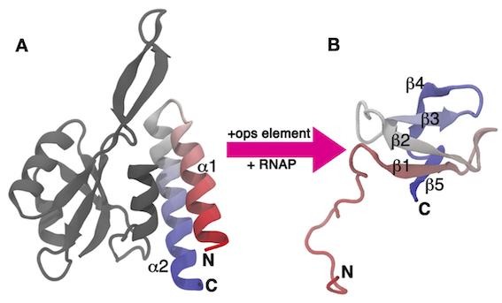
RfaH-CTD is simulated using a simplified, structure-based potential, called SMOG. The SMOG energy function has been designed to have two local minima corresponding to the β-barrel and α-helical states of RfaH-CTD. To achieve this goal, the SMOG energy function promotes native contacts, i.e. interactions that are present in the native structure(s). When using structure-based force fields, a function of the coordinates that is correlated with the energy of the system, such as the total number of native contacts, has been shown to be a good CV for enhanced-sampling simulations. Unfortunately, these types of CVs often involve a large number of atoms and are therefore computationally expensive to calculate at every step of the simulation. In this exercise, we will learn how to write and optimize these types of CVs.

In the data/exercise2 folder of the GitHub repository of this Masterclass, you will find:

• two PDB files of RfaH-CTD in the β-barrel (stateA.pdb) and α-helical (stateB.pdb) states;
• a topol.tpr file, which is needed to perform a MD simulation of this system with GROMACS;
• a template PLUMED input file (plumed.dat) to perform a metadynamics simulation using the total number of native contacts as CV. These contacts are defined using only the β-barrel conformation, which is the most populated state in the conditions we are simulating.

The provided PLUMED input file looks as follows:

Click on the labels of the actions for more information on what each action computes

# reconstruct molecule
WHOLEMOLECULESThis action is used to rebuild molecules that can become split by the periodic boundary conditions. More details ENTITY0the atoms that make up a molecule that you wish to align=1-330

# CA-RMSDs from the two reference conformations
# useful for monitoring the distance from the two metastable states
The WHOLEMOLECULES action with label  calculates somethingrmsd_A: RMSDCalculate the RMSD with respect to a reference structure. More details REFERENCEa file in pdb format containing the reference structure and the atoms involved in the CV=stateA.pdb TYPE the manner in which RMSD alignment is performed=OPTIMAL NOPBC ignore the periodic boundary conditions when calculating distances
The RMSD action with label rmsd_A calculates the following quantities:
 Quantity   
 Description  
rmsd_A.value
the RMSD distance between the instaneous structure and the reference structure/s that were inputrmsd_B: RMSDCalculate the RMSD with respect to a reference structure. More details REFERENCEa file in pdb format containing the reference structure and the atoms involved in the CV=stateB.pdb TYPE the manner in which RMSD alignment is performed=OPTIMAL NOPBC ignore the periodic boundary conditions when calculating distances

# list of 379 distances between atoms that are closer
# than 0.6 nm in the reference PDB file (stateA.pdb, β-barrel state)
The RMSD action with label rmsd_B calculates the following quantities:
 Quantity   
 Description  
rmsd_B.value
the RMSD distance between the instaneous structure and the reference structure/s that were inputd1: DISTANCECalculate the distance/s between pairs of atoms. More details ATOMSthe pair of atom that we are calculating the distance between=1,110 NOPBC ignore the periodic boundary conditions when calculating distances
The DISTANCE action with label d1 calculates the following quantities:
 Quantity   
 Description  
d1.value
the DISTANCE between this pair of atomsd2: DISTANCECalculate the distance/s between pairs of atoms. More details ATOMSthe pair of atom that we are calculating the distance between=1,115 NOPBC ignore the periodic boundary conditions when calculating distances
# __FILL__
The DISTANCE action with label d2 calculates the following quantities:
 Quantity   
 Description  
d2.value
the DISTANCE between this pair of atomsd379: DISTANCECalculate the distance/s between pairs of atoms. More details ATOMSthe pair of atom that we are calculating the distance between=239,265 NOPBC ignore the periodic boundary conditions when calculating distances

# list of 379 switching functions to define a contact from the distance between two atoms
The DISTANCE action with label d379 calculates the following quantities:
 Quantity   
 Description  
d379.value
the DISTANCE between this pair of atomsc1: CUSTOMCalculate a combination of variables using a custom expression. More details FUNCthe function you wish to evaluate=1-erf(x^4) ARGthe values input to this function=d1 PERIODICif the output of your function is periodic then you should specify the periodicity of the function=NO
The CUSTOM action with label c1 calculates the following quantities:
 Quantity   
 Description  
c1.value
an arbitrary functionc2: CUSTOMCalculate a combination of variables using a custom expression. More details FUNCthe function you wish to evaluate=1-erf(x^4) ARGthe values input to this function=d2 PERIODICif the output of your function is periodic then you should specify the periodicity of the function=NO
# __FILL__
The CUSTOM action with label c2 calculates the following quantities:
 Quantity   
 Description  
c2.value
an arbitrary functionc379: CUSTOMCalculate a combination of variables using a custom expression. More details FUNCthe function you wish to evaluate=1-erf(x^4) ARGthe values input to this function=d379 PERIODICif the output of your function is periodic then you should specify the periodicity of the function=NO

# sum of switching functions = total number of contacts
The CUSTOM action with label c379 calculates the following quantities:
 Quantity   
 Description  
c379.value
an arbitrary functioncv: COMBINECalculate a polynomial combination of a set of other variables. More details ARGthe values input to this function=c1,c2,c3,c4,c5,c6,c7,c8,c9,c10,c11,c12,c13,c14,c15,c16,c17,c18,c19,c20,c21,c22,c23,c24,c25,c26,c27,c28,c29,c30,c31,c32,c33,c34,c35,c36,c37,c38,c39,c40,c41,c42,c43,c44,c45,c46,c47,c48,c49,c50,c51,c52,c53,c54,c55,c56,c57,c58,c59,c60,c61,c62,c63,c64,c65,c66,c67,c68,c69,c70,c71,c72,c73,c74,c75,c76,c77,c78,c79,c80,c81,c82,c83,c84,c85,c86,c87,c88,c89,c90,c91,c92,c93,c94,c95,c96,c97,c98,c99,c100,c101,c102,c103,c104,c105,c106,c107,c108,c109,c110,c111,c112,c113,c114,c115,c116,c117,c118,c119,c120,c121,c122,c123,c124,c125,c126,c127,c128,c129,c130,c131,c132,c133,c134,c135,c136,c137,c138,c139,c140,c141,c142,c143,c144,c145,c146,c147,c148,c149,c150,c151,c152,c153,c154,c155,c156,c157,c158,c159,c160,c161,c162,c163,c164,c165,c166,c167,c168,c169,c170,c171,c172,c173,c174,c175,c176,c177,c178,c179,c180,c181,c182,c183,c184,c185,c186,c187,c188,c189,c190,c191,c192,c193,c194,c195,c196,c197,c198,c199,c200,c201,c202,c203,c204,c205,c206,c207,c208,c209,c210,c211,c212,c213,c214,c215,c216,c217,c218,c219,c220,c221,c222,c223,c224,c225,c226,c227,c228,c229,c230,c231,c232,c233,c234,c235,c236,c237,c238,c239,c240,c241,c242,c243,c244,c245,c246,c247,c248,c249,c250,c251,c252,c253,c254,c255,c256,c257,c258,c259,c260,c261,c262,c263,c264,c265,c266,c267,c268,c269,c270,c271,c272,c273,c274,c275,c276,c277,c278,c279,c280,c281,c282,c283,c284,c285,c286,c287,c288,c289,c290,c291,c292,c293,c294,c295,c296,c297,c298,c299,c300,c301,c302,c303,c304,c305,c306,c307,c308,c309,c310,c311,c312,c313,c314,c315,c316,c317,c318,c319,c320,c321,c322,c323,c324,c325,c326,c327,c328,c329,c330,c331,c332,c333,c334,c335,c336,c337,c338,c339,c340,c341,c342,c343,c344,c345,c346,c347,c348,c349,c350,c351,c352,c353,c354,c355,c356,c357,c358,c359,c360,c361,c362,c363,c364,c365,c366,c367,c368,c369,c370,c371,c372,c373,c374,c375,c376,c377,c378,c379 PERIODICif the output of your function is periodic then you should specify the periodicity of the function=NO

# metadynamics using "cv"
The COMBINE action with label cv calculates the following quantities:
 Quantity   
 Description  
cv.value
a linear compbinationmetad: METADUsed to performed metadynamics on one or more collective variables. More details ARGthe labels of the scalars on which the bias will act=cv ...
 # Deposit a Gaussian every 500 time steps, with initial height 
 # equal to 1.2 kJ/mol and bias factor equal to 60
 PACEthe frequency for hill addition=500 HEIGHTthe heights of the Gaussian hills=1.2 BIASFACTORuse well tempered metadynamics and use this bias factor=60 
 # Gaussian width (sigma) based on the CV fluctuations in unbiased run 
 SIGMAthe widths of the Gaussian hills=10.0
 # Gaussians will be written to file
 FILE a file in which the list of added hills is stored=HILLS
...

# print useful stuff
The METAD action with label metad calculates the following quantities:
 Quantity   
 Description  
metad.bias
the instantaneous value of the bias potentialPRINTPrint quantities to a file. More details ARGthe labels of the values that you would like to print to the file=cv,rmsd_A,rmsd_B,metad.bias STRIDE the frequency with which the quantities of interest should be output=500 FILEthe name of the file on which to output these quantities=COLVAR

# reconstruct molecule
WHOLEMOLECULESThis action is used to rebuild molecules that can become split by the periodic boundary conditions. More details ENTITY0the atoms that make up a molecule that you wish to align=1-330

# CA-RMSDs from the two reference conformations
The WHOLEMOLECULES action with label  calculates somethingrmsd_A: RMSDCalculate the RMSD with respect to a reference structure. More details REFERENCEa file in pdb format containing the reference structure and the atoms involved in the CV=../data/exercise2/stateA.pdb TYPE the manner in which RMSD alignment is performed=OPTIMAL NOPBC ignore the periodic boundary conditions when calculating distances
The RMSD action with label rmsd_A calculates the following quantities:
 Quantity   
 Description  
rmsd_A.value
the RMSD distance between the instaneous structure and the reference structure/s that were inputrmsd_B: RMSDCalculate the RMSD with respect to a reference structure. More details REFERENCEa file in pdb format containing the reference structure and the atoms involved in the CV=../data/exercise2/stateB.pdb TYPE the manner in which RMSD alignment is performed=OPTIMAL NOPBC ignore the periodic boundary conditions when calculating distances

The RMSD action with label rmsd_B calculates the following quantities:
 Quantity   
 Description  
rmsd_B.value
the RMSD distance between the instaneous structure and the reference structure/s that were inputcv: COORDINATIONCalculate coordination numbers. More details NOPBC ignore the periodic boundary conditions when calculating distances GROUPAFirst list of atoms=1,1,1,2,2,2,2,2,3,3,3,3,4,5,5,6,9,10,10,10,10,13,13,13,13,13,13,13,14,14,14,14,14,14,14,14,14,16,16,16,16,16,18,18,18,18,19,21,22,22,22,22,22,22,24,25,25,25,27,27,27,27,27,27,27,27,28,28,28,28,29,29,29,29,29,29,29,30,30,30,30,30,30,30,30,30,30,32,32,32,32,32,32,34,34,34,38,39,41,41,41,47,47,47,48,48,48,52,52,57,57,60,62,62,63,63,63,66,68,68,68,68,83,84,84,84,84,84,84,89,89,89,93,95,98,101,101,101,101,101,101,103,103,104,104,104,104,104,104,104,105,107,107,107,107,107,108,109,109,110,111,111,114,114,114,114,114,114,114,116,116,116,116,119,119,119,120,120,120,120,120,126,126,126,126,128,128,129,129,129,129,129,129,129,130,130,130,130,130,130,130,130,133,133,133,133,133,135,140,141,141,141,141,141,144,144,144,144,145,145,145,145,149,149,149,149,151,151,153,153,153,153,153,153,154,154,154,158,160,160,160,160,162,166,166,166,169,169,169,174,174,174,174,174,174,174,176,176,176,176,176,178,178,178,178,180,180,180,184,186,186,186,186,188,188,188,189,189,189,191,191,191,191,191,191,193,193,193,193,195,195,196,197,197,197,197,197,200,200,200,200,200,202,202,202,204,204,204,204,204,205,205,207,207,207,207,207,209,209,209,209,210,211,212,212,212,212,212,212,212,212,213,213,213,213,216,216,216,216,218,218,218,220,220,220,220,220,220,220,221,221,221,223,223,223,223,223,223,225,225,225,226,226,232,232,232,232,232,235,235,235,236,236,236,236,237,239,239,239 GROUPBSecond list of atoms (if empty, N*(N-1)/2 pairs in GROUPA are counted)=110,115,122,106,108,110,112,115,95,96,98,102,112,95,98,112,123,95,102,106,115,106,108,112,115,123,203,205,92,102,103,104,106,113,202,205,208,92,94,96,102,106,82,92,94,96,96,78,79,80,92,94,96,99,205,78,82,92,60,68,70,72,78,82,84,92,60,68,70,311,82,92,102,104,205,310,311,60,68,82,84,92,104,221,309,310,311,68,70,72,78,82,92,70,72,75,71,73,72,74,75,58,71,74,70,71,72,69,71,86,87,221,218,221,236,237,279,295,82,84,93,221,229,217,218,219,221,229,231,229,231,237,229,229,229,215,217,219,224,229,231,215,224,202,204,208,215,217,219,220,203,201,202,208,210,215,202,210,213,210,213,215,133,199,201,203,208,210,215,199,201,203,204,192,199,201,188,203,204,205,327,194,199,201,208,286,287,194,196,197,199,206,284,300,199,208,210,212,213,285,286,287,192,194,196,197,199,196,199,187,192,194,195,196,185,187,192,195,185,187,189,199,185,187,195,196,195,196,170,175,176,177,185,195,177,179,182,177,175,177,186,328,189,189,327,328,186,188,328,313,315,316,317,323,325,328,313,315,317,323,328,315,317,319,323,317,319,320,328,303,313,315,323,310,313,315,323,327,328,300,302,303,307,310,313,300,302,307,310,302,303,303,284,291,301,302,303,300,302,307,310,313,300,307,310,300,302,307,310,313,310,313,281,283,291,300,310,281,283,285,291,287,267,267,270,274,281,283,285,287,288,267,270,287,288,274,278,281,291,278,279,281,278,279,281,283,291,293,300,278,279,293,264,266,274,277,278,281,266,267,268,268,271,266,268,274,277,278,266,274,278,274,277,278,279,279,256,258,265 PAIR Pair only 1st element of the 1st group with 1st element in the second, etc SWITCHThis keyword is used if you want to employ an alternative to the continuous switching function defined above. Options for this keyword are explained in the documentation for LESS_THAN.={CUSTOM FUNC=1-erf(x^4) R_0=1.0}

# metadynamics parameters
The COORDINATION action with label cv calculates the following quantities:
 Quantity   
 Description  
cv.value
the value of the coordinationmetad: METADUsed to performed metadynamics on one or more collective variables. More details ARGthe labels of the scalars on which the bias will act=cv ...
  # Deposit a Gaussian every 500 time steps, with initial height
  # equal to 1.2 kJ/mol and bias factor equal to 60
  PACEthe frequency for hill addition=500 HEIGHTthe heights of the Gaussian hills=1.2 BIASFACTORuse well tempered metadynamics and use this bias factor=60
  # Gaussian width (sigma) based on the CV fluctuations in unbiased run
  SIGMAthe widths of the Gaussian hills=2.0
  # Store MetaD bias potential on a grid
  GRID_MINthe lower bounds for the grid=0 GRID_MAXthe upper bounds for the grid=400
  # Gaussians will be written to file
  FILE a file in which the list of added hills is stored=HILLS
  # Multiple time stepping
  STRIDEthe frequency with which the forces due to the bias should be calculated=4
...

# Energy drift
The METAD action with label metad calculates the following quantities:
 Quantity   
 Description  
metad.bias
the instantaneous value of the bias potentialEFFECTIVE_ENERGY_DRIFTPrint the effective energy drift More details PRINT_STRIDEfrequency to which output the effective energy drift on FILE=500 FILEfile on which to output the effective energy drift=COLVAR_ENE

# print useful stuff
PRINTPrint quantities to a file. More details ARGthe labels of the values that you would like to print to the file=cv,rmsd_A,rmsd_B,metad.bias STRIDE the frequency with which the quantities of interest should be output=500 FILEthe name of the file on which to output these quantities=COLVAR

The objectives of this exercise are to:

1. optimize the distance-based CV provided in the template PLUMED input file. The user should report the speedup obtained with the optimized CV with respect to the one defined in the provided input file;
2. optimize the performances of well-tempered metadynamics.
3. evaluate the stability of the β-barrel state of RfaH-CTD (with error estimate). Have a look at this earlier lessonr for more info.

Suggestions:

• the users should consult the PLUMED manual in order to optimize the proposed CV;
• the COORDINATION CV can be defined using a custom switching function, whose calculation can be made faster by using AsmJit. For more information, have a look here;
• try Multiple time stepping to apply the metadynamics bias every 2 or 4 steps using the STRIDE option on the METAD line.

Please keep in mind that:

• SMOG is significantly less computational demanding than all-atoms, explicit solvent force fields. However, the simulation of this system might take a few hours, so allocate enough time to complete this exercise;
• due to the special nature of the force field, please execute GROMACS using the following command: gmx mdrun -plumed plumed.dat -ntomp 4 -noddcheck. You can adjust the number of CPU cores you want to use (here 4, OpenMP parallelization), based on the available resources. The system is not particularly big, therefore using a large number of cores might be inefficient.