
Ab-initio Metadynamics: Small Silver Cluster
In the same way as we analyzed the toy model, we can also obtain the free energy profile using an Ab-initio calculator. In this part of the tutorial, we show how to find the free energy surface of an Ag-6 cluster presented in the paper D. Sucerquia et. al., JCP, 2022. There, we showed that this cluster is the smallest silver cluster where entropic effects at room temperature boost the non-planar isomer probability to a competing state.
Collective variables
To obtain a proper exploration of the different states of the silver cluster, we can use the coordination number (C) and the radius of gyration (R) as collective variables. These Collective variables are defined as
\[C= \sum_{i=1}^{N_a} \sum_{j\ne i}\frac{1-(r_{ij}/d)^8}{1-(r_{ij}/d)^{16}},\]and
\[R= \left(\frac{\sum_i^N |{\color{black}{\bf r}}_i - {\color{black}{\bf r}}_{CM}|^2}{N_a}\right)^{1/2},\]where $r_i$ is the position of atom $i$, $r_{CM}$ is the center of mass of the cluster and $N_a$ is the number of atoms of the cluster. This CV gives information about how disperse the system is with respect to the center of mass. $C$ and $R$ enable extracting information about the shape of the cluster and permit differentiating the free-energy minima found by DFT optimization, which are expected to be metastable states in the free energy landscape.
By performing short WT-MTD along these CVs, we noticed that there were isomers with broken bonds or that formed linear clusters, which are not of interest in the isomerisation process. Therefore, there are regions of the space that are thermodynamically insignificant. Considering how expensive Ab-initio calculations are, and to avoid enhancing the exploration toward these regions, we created a new set of CVs (CV1 and CV2) that are a rotation of C and R, which allow us to easily apply a constraint, as in the previous example. The rotated CVs are defined as
\[CV 1 = 0.99715 C − 0.07534Å^{−1} R\]and
\[CV 2 = 0.07534 C + 0.99715Å^{−1} R\]Using this CV setup for WT-MTD, we added walls using repulsive semi-harmonic potentials that act when CV1 is lower than 8 with harmonic constant 10 eV and values of CV2 greater than 3.3 with harmonic constant 50 eV.
Running the Simulation
| WARNING |
|---|
The aim of this tutorial is to show an example of the capabilities of the ASE-PLUMED calculatory. To obtain a full reconstruction of the free energy surface, metadynamics must to run for a long time to reach convergence. This could take many hours (or even days) to be completed. The code presented here runs for 1000 time steps, which gives an estimate of the free energy surface, although real convergence cannot yet be guaranteed. For more details on how we achieved convergence in this case, check the paper D. Sucerquia et. al., JCP, 2022. For longer simulations, you have to change the argument of the function run in the last line, and you might need to use High Performance Computing in order to complete it in a feasible time. |
You need to create a file called plumedSC.dat containing the lines,
UNITSThis command sets the internal units for the code. More details LENGTHthe units of lengths=A TIMEthe units of time=0.0101805 ENERGYthe units of energy=96.4853329 c: COORDINATIONCalculate coordination numbers. This action has hidden defaults. More details GROUPAFirst list of atoms=1-6 GROUPBSecond list of atoms (if empty, N*(N-1)/2 pairs in GROUPA are counted)=1-6 R_0The r_0 parameter of the switching function=2.8 r: GYRATIONCalculate the radius of gyration, or other properties related to it. More details ATOMSthe group of atoms that you are calculating the Gyration Tensor for=1-6 rrot: COMBINECalculate a polynomial combination of a set of other variables. More details ARGthe values input to this function=c,r COEFFICIENTS the coefficients of the arguments in your function=0.07534,0.99715 PERIODICif the output of your function is periodic then you should specify the periodicity of the function=NO crot: COMBINECalculate a polynomial combination of a set of other variables. More details ARGthe values input to this function=c,r COEFFICIENTS the coefficients of the arguments in your function=0.99715,-0.07534 PERIODICif the output of your function is periodic then you should specify the periodicity of the function=NO UPPER_WALLSDefines a wall for the value of one or more collective variables, More details ARGthe arguments on which the bias is acting=rrot ATthe positions of the wall=3.3 KAPPAthe force constant for the wall=50 LOWER_WALLSDefines a wall for the value of one or more collective variables, More details ARGthe arguments on which the bias is acting=crot ATthe positions of the wall=8. KAPPAthe force constant for the wall=10 METADUsed to performed metadynamics on one or more collective variables. More details ARGthe labels of the scalars on which the bias will act=crot,rrot SIGMAthe widths of the Gaussian hills=0.3,0.03 HEIGHTthe heights of the Gaussian hills=0.2 PACEthe frequency for hill addition=100 BIASFACTORuse well tempered metadynamics and use this bias factor=100 FILE a file in which the list of added hills is stored=HILLS FLUSHThis command instructs plumed to flush all the open files with a user specified frequency. More details STRIDEthe frequency with which all the open files should be flushed=100
Once this file is created, we can start the simulation from one of the DFT-optimized configurations, here called isomerSC.xyz. Note that for this part of the tutorial you need to set up GPAW, which is a DFT code. You can choose the QM code that you prefer. This can be done as shown in the file MTD-SC.py:
from ase.md.velocitydistribution import MaxwellBoltzmannDistribution
from ase.md.nvtberendsen import NVTBerendsen
from gpaw import MixerDif, FermiDirac, GPAW
from ase.calculators.plumed import Plumed
from ase.io import read
from ase import Atoms
from ase import units


pos = read("isomerSC.xyz").get_positions()

setup = open("plumedSC.dat", "r").read().splitlines()

T = 100
timestep = 5 * units.fs
taut = 50 * units.fs

atoms = Atoms('Ag6', pos)

MaxwellBoltzmannDistribution(atoms, temperature_K=T)

p = atoms.get_momenta()
psum = p.sum(axis=0) / float(len(p))
p = p - psum
atoms.set_momenta(p)

a = 16

atoms.set_cell([a, a, a])
atoms.set_pbc(True)
atoms.center()

atoms.calc = Plumed(GPAW(h=0.2,
                         mode='lcao',
                         basis='pvalence.dz',
                         xc='PBE',
                         spinpol=True,
                         nbands=-4,
                         occupations=FermiDirac(0.05),
                         parallel=dict(augment_grids=True),
                         mixer=MixerDif(beta=0.25, nmaxold=3, weight=50.0),
                         symmetry='off'),
                    input=setup,
                    timestep=timestep,
                    atoms=atoms,
                    kT=units.kB*T)

dyn = NVTBerendsen(atoms, timestep, temperature_K=T, taut=taut, fixcm=False,
                   trajectory='trajectory.traj')

dyn.run(1000)
After running this same code but changing the temperature and the number of time steps, you can obtain the free energy surfaces shown in Figure 4.
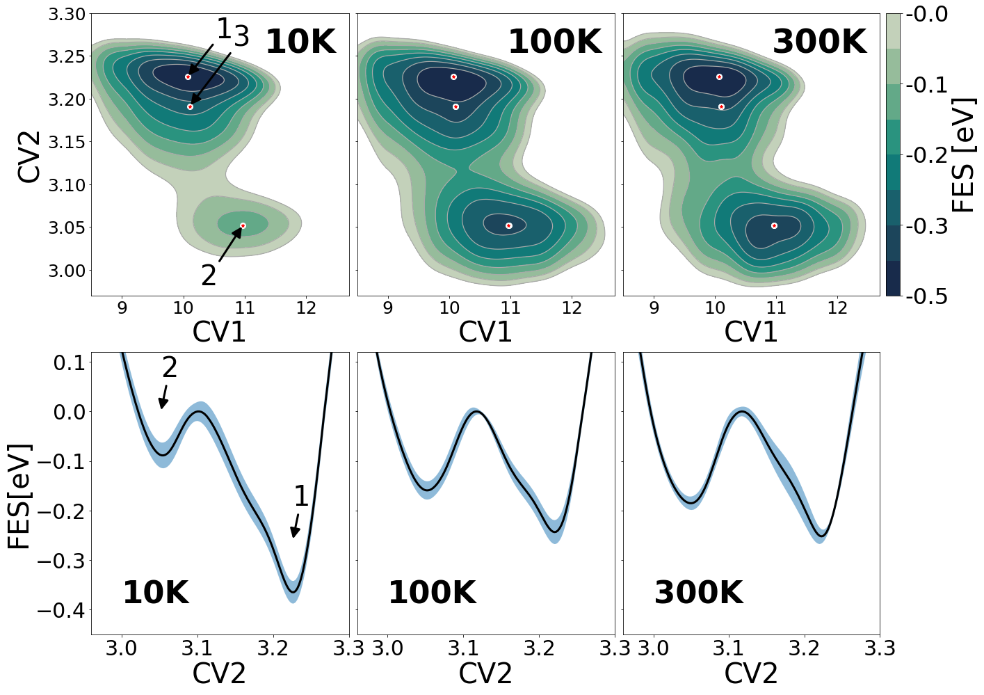
Figure 4. Free energy surface of a Ag6 cluster at three different temperatures.