
Molecular Dynamics Simulation
Let’s start with a Langevin simulation without bias. In LJ dimensionless reduced units (assuming $\epsilon$ = 1 eV, $\sigma$ = 1 $\textrm Å$ and m = 1 a.m.u), the parameters of the simulation are $k_\text{B}T=0.1$, friction coefficient fixed equal to 1 and a time step of 0.005.
In principle, the system should explore all the configuration space
due to thermal fluctuations. However, we can see that the system remains in the
same conformational state, even when we simulate for a long time. This happens because the system gets trapped in a local minimum and a
complete exploration of the configuration
space is too expensive computationally. Figure 2 -blue
dots- shows the trajectory obtained from the following unbiased
Molecular Dynamics MD.py:
from ase.calculators.lj import LennardJones
from ase.calculators.plumed import Plumed
from ase.constraints import FixedPlane
from ase.md.langevin import Langevin
from ase.io import read
from ase import units


timestep = 0.005

ps = 1000 * units.fs
setup = open("plumedLJ.dat", "r").read().splitlines()

atoms = read('isomer.xyz')
# Constraint to keep the system in a plane
cons = [FixedPlane(i, [0, 0, 1]) for i in range(7)]
atoms.set_constraint(cons)
atoms.set_masses([1, 1, 1, 1, 1, 1, 1])

atoms.calc = Plumed(calc=LennardJones(rc=3., r0=2.5, smooth=True),
                    input=setup,
                    timestep=timestep,
                    atoms=atoms,
                    kT=0.1)

dyn = Langevin(atoms, timestep, temperature_K=0.1/units.kB, friction=1,
               fixcm=False, trajectory='UnbiasMD.xyz')

dyn.run(100000)
Where plumedLJ.dat
contains the next information:
UNITSThis command sets the internal units for the code. More details LENGTHthe units of lengths=A TIMEthe units of time=0.0101805 ENERGYthe units of energy=96.4853329 c1: COORDINATIONNUMBERCalculate the coordination numbers of atoms so that you can then calculate functions of the distribution of This action is a shortcut. More details SPECIESthe list of atoms for which the symmetry function is being calculated and the atoms that can be in the environments=1-7 MOMENTSthe list of moments that you would like to calculate=2-3 SWITCHthe switching function that it used in the construction of the contact matrix. Options for this keyword are explained in the documentation for LESS_THAN.={RATIONAL R_0=1.5 NN=8 MM=16} PRINTPrint quantities to a file. More details ARGthe labels of the values that you would like to print to the file=c1.* STRIDE the frequency with which the quantities of interest should be output=100 FILEthe name of the file on which to output these quantities=COLVAR FLUSHThis command instructs plumed to flush all the open files with a user specified frequency. More details STRIDEthe frequency with which all the open files should be flushed=1000
This simulation starts from the configuration of minimum energy, whose
coordinates are imported from isomerLJ.xyz.
As you can see in Figure 2, the
system remains around that state and it does not jump to the other
isomers, thereby not fully sampling all possible
configurations of the system. It is therefore necessary to use an enhanced
sampling method.
In this tutorial, we implement Well-Tempered Metadynamics.
| WARNING |
|---|
Note that in the plumed setup, there is a line with the keyword UNITS, which is necessary because all parameters and output files are assumed to be in plumed internal units. This line is important to maintain the units of all plumed parameters and outputs in ASE units. You can ignore this line if you are aware of the unit conversion. |
Post Processing Analysis
Once you have the trajectory of an MD simulation and you want to compute a set of
CVs of that trajectory, you can reconstruct the plumed files without running
again the simulation. As an example, let’s use the trajectory created in
the last example to rewrite the COLVAR file with the code postpro.py:
from ase.calculators.idealgas import IdealGas
from ase.calculators.plumed import Plumed
from ase.io import read
from ase import units


traj = read('UnbiasMD.xyz', index=':')

atoms = traj[0]

timestep = 0.005
ps = 1000 * units.fs
setup = open("plumedLJ.dat", "r").read().splitlines()

# IdealGas is a calculator that removes all ineractions.
calc = Plumed(calc=IdealGas(),
              input=setup,
              timestep=timestep,
              atoms=atoms,
              kT=0.1)

calc.write_plumed_files(traj)
This code, as well as the previous one, generates a file called COLVAR with the value of the CVs. All PLUMED files begin with a header that describes the fields that it contains. In this case, the header looks like:
$ head -n 2 COLVAR
#! FIELDS time c1.moment-2 c1.moment-3
0.000000 0.757954 1.335796
As you can see, the first column corresponds to the time, the second one is the second central moment (SCM) and the third column is the third central moment (TCM). When we plot this trajectory in the space of these CVs (that is, the second and third columns) we obtain this result:
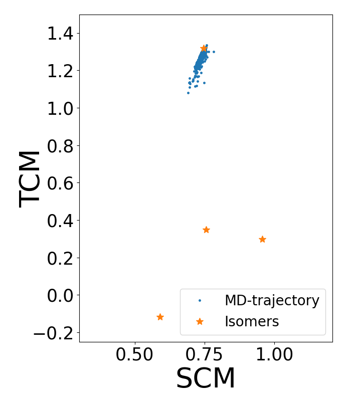
Figure 2. Unbiased MD trajectory (blue dots) in the space of the collective variables second and third central moment. Orange stars represent the location of the local minima isomers of the LJ cluster in this space.
Note that the system remains confined in the same stable state. Therefore, the MD simulation is too short and it is not possible to explore all configurations or to obtain a statistical study of the possible configurations of the system. An alternative is to use an enhanced sampling method. In this case, we implement Well-Tempered Metadynamics for reconstructing the Free Energy Surface (FES).