Well-Tempered Metadynamics Simulation

The Well-Tempered Metadynamics method is an enhanced sampling method described in the Theory section. It adds external energy for pushing the system to explore different conformations. to avoid atom dissociation, we add a restraint to the system. This restriction consists of a semi-harmonic potential with the form

\[V(d_i)= \begin{array}{ll} k (d_i - r_w)^2 & \text{if }d_i>2 \\ 0 & \text{otherwise} \end{array} ~,\]

where $k$ is a constraint, in this case being 1000; $r_w$ is the location of the constraint, that we choose to be 2 (in LJ dimensionless reduced units); $d_i$ is the distance of each atom to the center of mass. Note that this potential does not do anything if the distance between the atom and the center of mass is lower than $r_w$, but if it is greater this potential begins to exert a force over the atoms and to avoid dissociation. This is defined with the keyword UPPER_WALLS in the plumed setup.

An example PLUMED file with the information of the constraints (also called walls) and the coordinates you want to bias can be found here (plumedMTD-LJ.dat):

Click on the labels of the actions for more information on what each action computes

UNITSThis command sets the internal units for the code. More details LENGTHthe units of lengths=A TIMEthe units of time=0.0101805 ENERGYthe units of energy=96.4853329
The UNITS action with label  calculates somethingCOMCalculate the center of mass for a group of atoms. More details ATOMSthe list of atoms which are involved the virtual atom's definition=1-7 LABELa label for the action so that its output can be referenced in the input to other actions=comThe COM action with label com calculates the following quantities: Quantity    Type    Description  
com atoms virtual atom calculated by COM action
DISTANCECalculate the distance/s between pairs of atoms. More details ATOMSthe pair of atom that we are calculating the distance between=1,com LABELa label for the action so that its output can be referenced in the input to other actions=d1The DISTANCE action with label d1 calculates the following quantities: Quantity    Type    Description  
d1 scalar the DISTANCE between this pair of atoms
UPPER_WALLSDefines a wall for the value of one or more collective variables, More details ARGthe arguments on which the bias is acting=d1 ATthe positions of the wall=2.0 KAPPAthe force constant for the wall=100.
DISTANCECalculate the distance/s between pairs of atoms. More details ATOMSthe pair of atom that we are calculating the distance between=2,com LABELa label for the action so that its output can be referenced in the input to other actions=d2The DISTANCE action with label d2 calculates the following quantities: Quantity    Type    Description  
d2 scalar the DISTANCE between this pair of atoms
UPPER_WALLSDefines a wall for the value of one or more collective variables, More details ARGthe arguments on which the bias is acting=d2 ATthe positions of the wall=2.0 KAPPAthe force constant for the wall=100.
DISTANCECalculate the distance/s between pairs of atoms. More details ATOMSthe pair of atom that we are calculating the distance between=3,com LABELa label for the action so that its output can be referenced in the input to other actions=d3The DISTANCE action with label d3 calculates the following quantities: Quantity    Type    Description  
d3 scalar the DISTANCE between this pair of atoms
UPPER_WALLSDefines a wall for the value of one or more collective variables, More details ARGthe arguments on which the bias is acting=d3 ATthe positions of the wall=2.0 KAPPAthe force constant for the wall=100.
DISTANCECalculate the distance/s between pairs of atoms. More details ATOMSthe pair of atom that we are calculating the distance between=4,com LABELa label for the action so that its output can be referenced in the input to other actions=d4The DISTANCE action with label d4 calculates the following quantities: Quantity    Type    Description  
d4 scalar the DISTANCE between this pair of atoms
UPPER_WALLSDefines a wall for the value of one or more collective variables, More details ARGthe arguments on which the bias is acting=d4 ATthe positions of the wall=2.0 KAPPAthe force constant for the wall=100.
DISTANCECalculate the distance/s between pairs of atoms. More details ATOMSthe pair of atom that we are calculating the distance between=5,com LABELa label for the action so that its output can be referenced in the input to other actions=d5The DISTANCE action with label d5 calculates the following quantities: Quantity    Type    Description  
d5 scalar the DISTANCE between this pair of atoms
UPPER_WALLSDefines a wall for the value of one or more collective variables, More details ARGthe arguments on which the bias is acting=d5 ATthe positions of the wall=2.0 KAPPAthe force constant for the wall=100.
DISTANCECalculate the distance/s between pairs of atoms. More details ATOMSthe pair of atom that we are calculating the distance between=6,com LABELa label for the action so that its output can be referenced in the input to other actions=d6The DISTANCE action with label d6 calculates the following quantities: Quantity    Type    Description  
d6 scalar the DISTANCE between this pair of atoms
UPPER_WALLSDefines a wall for the value of one or more collective variables, More details ARGthe arguments on which the bias is acting=d6 ATthe positions of the wall=2.0 KAPPAthe force constant for the wall=100.
DISTANCECalculate the distance/s between pairs of atoms. More details ATOMSthe pair of atom that we are calculating the distance between=7,com LABELa label for the action so that its output can be referenced in the input to other actions=d7The DISTANCE action with label d7 calculates the following quantities: Quantity    Type    Description  
d7 scalar the DISTANCE between this pair of atoms
UPPER_WALLSDefines a wall for the value of one or more collective variables, More details ARGthe arguments on which the bias is acting=d7 ATthe positions of the wall=2.0 KAPPAthe force constant for the wall=100.
c1The COORDINATIONNUMBER action with label c1 calculates the following quantities: Quantity    Type    Description  
c1 vector the coordination numbers of the specified atoms: COORDINATIONNUMBERCalculate the coordination numbers of atoms so that you can then calculate functions of the distribution of This action is a shortcut. More details SPECIESthe list of atoms for which the symmetry function is being calculated and the atoms that can be in the environments=1-7 MOMENTSthe list of moments that you would like to calculate=2-3 SWITCHthe switching function that it used in the construction of the contact matrix. Options for this keyword are explained in the documentation for LESS_THAN.={RATIONAL R_0=1.5 NN=8 MM=16}
# PLUMED interprets the command:
# c1: COORDINATIONNUMBER SPECIES=1-7 MOMENTS=2-3 SWITCH={RATIONAL R_0=1.5 NN=8 MM=16}
# as follows (Click the red comment above to revert to the short version of the input):
c1_grpThe GROUP action with label c1_grp calculates the following quantities: Quantity    Type    Description  
c1_grp atoms indices of atoms specified in GROUP: GROUPDefine a group of atoms so that a particular list of atoms can be referenced with a single label in definitions of CVs or virtual atoms. More details ATOMSthe numerical indexes for the set of atoms in the group=1-7
c1_matThe CONTACT_MATRIX action with label c1_mat calculates the following quantities: Quantity    Type    Description  
c1_mat matrix a matrix containing the weights for the bonds between each pair of atoms: CONTACT_MATRIXAdjacency matrix in which two atoms are adjacent if they are within a certain cutoff. More details GROUPspecifies the list of atoms that should be assumed indistinguishable=1-7 SWITCHthe input for the switching function that acts upon the distance between each pair of atoms. Options for this keyword are explained in the documentation for LESS_THAN.={RATIONAL R_0=1.5 NN=8 MM=16}
c1_onesThe CONSTANT action with label c1_ones calculates the following quantities: Quantity    Type    Description  
c1_ones vector the constant value that was read from the plumed input: ONESCreate a constant vector with all elements equal to one More details SIZEthe number of ones that you would like to create=7
c1The MATRIX_VECTOR_PRODUCT action with label c1 calculates the following quantities: Quantity    Type    Description  
c1 vector the vector that is obtained by taking the product between the matrix and the vector that were input: MATRIX_VECTOR_PRODUCTCalculate the product of the matrix and the vector More details  ARGthe label for the matrix and the vector/scalar that are being multiplied=c1_mat,c1_ones
c1_caverageThe MEAN action with label c1_caverage calculates the following quantities: Quantity    Type    Description  
c1_caverage scalar the mean of all the elements in the input vector: MEANCalculate the arithmetic mean of the elements in a vector More details ARGthe values input to this function=c1 PERIODICif the output of your function is periodic then you should specify the periodicity of the function=NO
c1_diffpow-2The CUSTOM action with label c1_diffpow-2 calculates the following quantities: Quantity    Type    Description  
c1_diffpow-2 vector the vector obtained by doing an element-wise application of an arbitrary function to the input vectors: CUSTOMCalculate a combination of variables using a custom expression. More details ARGthe values input to this function=c1,c1_caverage PERIODICif the output of your function is periodic then you should specify the periodicity of the function=NO FUNCthe function you wish to evaluate=(x-y)^2
c1_moment-2The MEAN action with label c1_moment-2 calculates the following quantities: Quantity    Type    Description  
c1_moment-2 scalar the mean of all the elements in the input vector: MEANCalculate the arithmetic mean of the elements in a vector More details ARGthe values input to this function=c1_diffpow-2 PERIODICif the output of your function is periodic then you should specify the periodicity of the function=NO
c1_diffpow-3The CUSTOM action with label c1_diffpow-3 calculates the following quantities: Quantity    Type    Description  
c1_diffpow-3 vector the vector obtained by doing an element-wise application of an arbitrary function to the input vectors: CUSTOMCalculate a combination of variables using a custom expression. More details ARGthe values input to this function=c1,c1_caverage PERIODICif the output of your function is periodic then you should specify the periodicity of the function=NO FUNCthe function you wish to evaluate=(x-y)^3
c1_moment-3The MEAN action with label c1_moment-3 calculates the following quantities: Quantity    Type    Description  
c1_moment-3 scalar the mean of all the elements in the input vector: MEANCalculate the arithmetic mean of the elements in a vector More details ARGthe values input to this function=c1_diffpow-3 PERIODICif the output of your function is periodic then you should specify the periodicity of the function=NO
# --- End of included input --- METADUsed to performed metadynamics on one or more collective variables. More details ARGthe labels of the scalars on which the bias will act=c1.* HEIGHTthe heights of the Gaussian hills=0.05 PACEthe frequency for hill addition=500 SIGMAthe widths of the Gaussian hills=0.1,0.1 GRID_MINthe lower bounds for the grid=-1.5,-1.5 GRID_MAXthe upper bounds for the grid=2.5,2.5 GRID_BINthe number of bins for the grid=500,500 BIASFACTORuse well tempered metadynamics and use this bias factor=5 FILE a file in which the list of added hills is stored=HILLS

The Well-Tempered Metadynamics simulation can be run using the code MTD.py:

from ase.calculators.lj import LennardJones
from ase.calculators.plumed import Plumed
from ase.constraints import FixedPlane
from ase.md.langevin import Langevin
from ase.io import read
from ase import units

timestep = 0.005
ps = 1000 * units.fs

setup = open("plumedMTD-LJ.dat", "r").read().splitlines()

atoms = read('isomerLJ.xyz')
cons = [FixedPlane(i, [0, 0, 1]) for i in range(7)]
atoms.set_constraint(cons)
atoms.set_masses([1, 1, 1, 1, 1, 1, 1])

atoms.calc = Plumed(calc=LennardJones(rc=3., r0=2.5, smooth=True),
                    input=setup,
                    timestep=timestep,
                    atoms=atoms,
                    kT=0.1)

dyn = Langevin(atoms, timestep, temperature_K=0.1/units.kB, friction=1,
               fixcm=False, trajectory='MTD.traj')

dyn.run(500000)

Note that Well-Tempered Metadynamics requires the value of the temperature according to equation (2) . Then, it is necessary to define the kT argument of the calculator. SIGMA and PACE are the standard deviation of the Gaussians and the deposition interval in terms of the number of steps ($\tau$ in equation (1)), respectively. HEIGHT and BIASFACTOR are the maximum height of the Gaussians (W) and the $\gamma$ factor of equation (2), respectively.

In this case, the Lennard-Jones calculator computes the forces between atoms, namely, ${\bf F}_i$ forces in equation (3). Likewise, you can use any preferred ASE calculator in place of the LJ calculator used here.

When one runs a metadynamics simulation, Plumed generates an output file called HILLS that contains the information of the deposited Gaussians. You can reconstruct the free energy by yourself or can use the plumed tool sum_hills. The simplest way of using it is:

$ plumed sum_hills --hills HILLS

After this, Plumed creates a fes.dat file with the free energy surface (FES) reconstructed. The FES of this example is plotted using plotterFES.py:

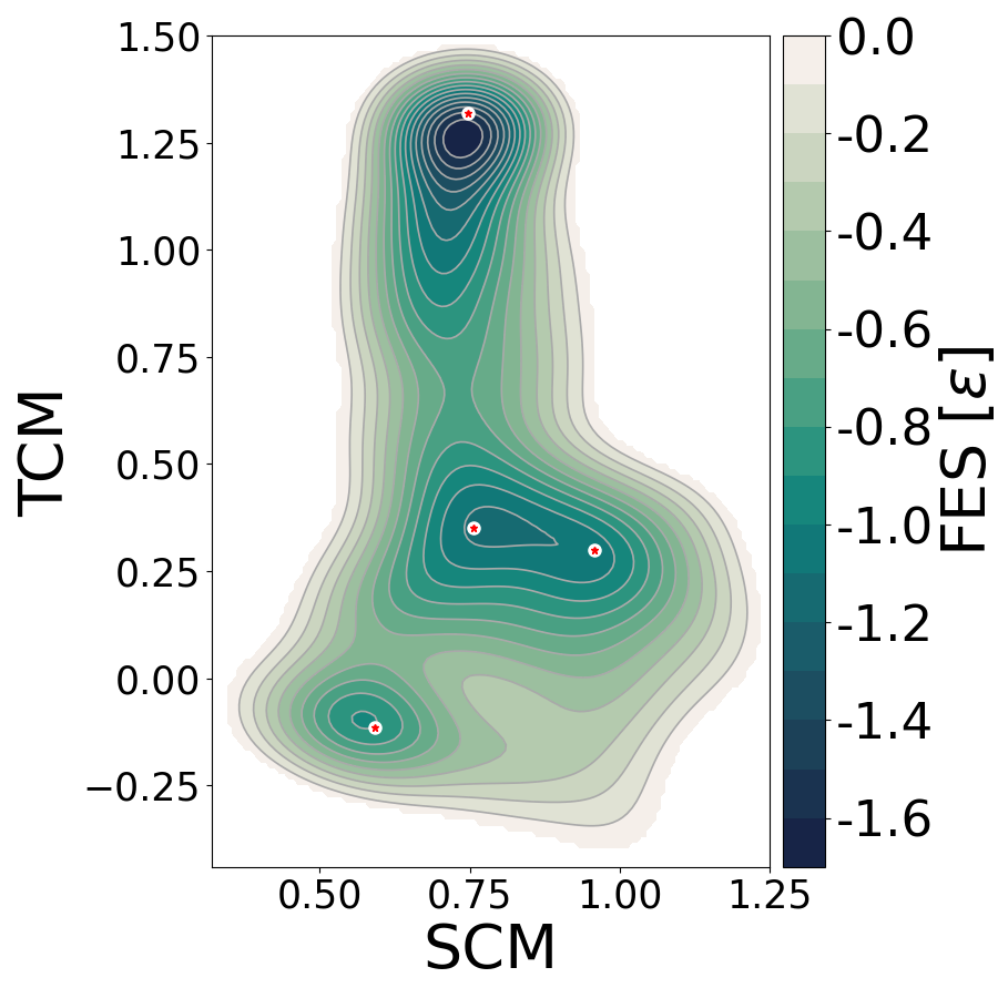
Figure 3. Free energy surface (LJ units) in the space of the collective variables second and third central moment. Orange stars represent the location of the local minima isomers of the LJ cluster in this space.

Note that bias is added over all states, meaning that the system jumped from one state to another and gave a complete reconstruction of the free energy surface.

PLUMED-TUTORIALS

A collaborative, community-driven learning ecosystem

Well-Tempered Metadynamics Simulation

← Unbiased simulation and Postprocessing

Restart a simulation →

Ab-initio: Small Silver Cluster →

Quantity	Type	Description
com	atoms	virtual atom calculated by COM action